Getting and using OSM data
In this section we will focus on two basic yet necessary steps to work with OpenStreetMap (OSM) data for transport research:
- Downloading OSM data using command line
- Plotting OSM data as a method to grasp data and its structure
The ability to download OSM data via command line might sound more intimidating compared to Graphical User Interface (GUI) but it can provide a much more flexible approach to working with OSM, including data analysis which will be covered in the later sections.
Before we begin, I want to remind the basic structure of OSM tags (if you need a more detailed refresher, see “Getting started with open data on transport infrastructure”). A tag consists of a key and a value (key = value). A value can take both numeric and character values. The tags and their meanings that will be used in this notebook are outlined in the Table 1.| Tag | Meaning |
|---|---|
| highway | It indicates the road type. |
| foot | Provides information on the legal access for pedestrians. |
| access | Provides information on the legal permissions and restrictions. |
| service | Provides additional information on the services (roads, businesses). |
| Note: | |
| Links to relevant OSM wiki pages: | |
| 1 highway: https://wiki.openstreetmap.org/wiki/Key:highway | |
| 2 foot: https://wiki.openstreetmap.org/wiki/Key:foot | |
| 3 access: https://wiki.openstreetmap.org/wiki/Key:access | |
| 4 service: https://wiki.openstreetmap.org/wiki/Key:service |
Getting OSM data
Here we will learn how to download OSM data using osmextract package in
R. osmextract that has been developed to make OSM data more
accessible. It returns a well-formatted OSM data that can be used as
part of a reproducible research. Another advantage of
osmextract over, for example, osmdata is its
capability to download large datasets. To learn more about this, check
out its website.
osmextract offers several different functions to
download, read, and translate OSM data, there is no one best function
and the choice depends on, for example, whether you already have a
dataset that needs to be translated. In this section it will be assumed
that you want to download the OSM data. For this, two functions will be
demonstrated:
- oe_get()
- oe_get_network()
In this section we will only touch upon the basics, so if you want to
learn more about the package, go through the Get
Started article published on the osmextract
website.
# Before we start, we need to load the libraries that we will be using throughout the practical.
library(tidyverse)
library(sf)
library(osmextract)
library(tmap)

# If you do not have these libraries installed, then run the following code (uncomment first) and load them again:
# pkgs = c("tidyverse",
#          "sf",
#          "osmextract")
# install.packages(pkgs)
Another important note: to increase the reproducibility of the results, we use pre-downloaded datasets throughout this codebook. Hence, the size of your dataset might differ (be more up-to-date) than the one used here. If you want to reproduce the same results, use the chunk of code below to get your data, otherwise skip it and proceed to “Downloading OSM network…” sections.
url1 = "https://github.com/udsleeds/openinfra/releases/download/v0.1/leeds_net_walking.geojson"
download.file(url1,
              destfile = "leeds_net_walking.geojson")
url2 = "https://github.com/udsleeds/openinfra/releases/download/v0.1/leeds.geojson"
download.file(url2,
              destfile = "leeds.geojson")
url3 = "https://github.com/udsleeds/openinfra/releases/download/v0.1/leeds_tn.geojson"
download.file(url3,
              destfile = "leeds_tn.geojson")

leeds_net_walking = sf::read_sf("leeds_net_walking.geojson")
leeds = sf::read_sf("leeds.geojson")
leeds_tn = sf::read_sf("leeds_tn.geojson")
Downloading OSM network with osmextract::oe_get()
oe_get() is perhaps the core function in the package and
the one I would recommend starting from because it is quite
straightforward once introduced, yet versatile enough to meet the needs
of an advanced user.
?osmextract::oe_get() # Documentation of a function

# The first step is to define the place. In this case it is Leeds.
# A useful function is oe_match_pattern() to search for patterns in a provider's database. It is helpful in indicating a correct region name for a given provider.
osmextract::oe_match_pattern("leeds")
osmextract::oe_match_pattern("yorkshire") # "yorkshire" is associated with several different geographic zones.
region_leeds = "Leeds" # Note the capital L. The function in which the object will be used is not case sensitive but I would still recommend using the exact string to minimize the likelihood of an error.

leeds = osmextract::oe_get(
  place = region_leeds,
  provider = "bbbike", # Indicates the provider; default is geofabrik
  layer = "lines", # Default; returns linestring geometries (highways, waterways, aerialways)
  force_download = TRUE, # Updates the previously downloaded .osm.pbf file (default is FALSE)
  force_vectortranslate = TRUE # Forces the vectorization of a .pbf file to .gpbf even if there is a .gpbf file with the same name (default = FALSE)
)- If you are curious, you can check out what happens when you input
“leeds” instead of “Leeds” if the provider is not specified (uncomment
leeds_testobject in the code chunk below).
# leeds_test = osmextract::oe_get(
#   place = "leeds",
#   force_download = TRUE,
#   force_vectortranslate = TRUE
# )

#> No exact match found for place = leeds and provider = geofabrik. Best match is Laos. Checking the other providers. An exact string match was found using provider = bbbike.
# Even though there was no exact string match (i.e., leeds) in a default provider, it still returned the dataset we needed by switching the provider. In this case it is fine, but it could cause problems for, for instance, "yorkshire" (test it out if you are up for a little challenge).
Downloading OSM network with osmextract::oe_get_network()
This function is a quick and useful way to return a desired road
network. However, it is important to point out that (compared to
oe_get()) some filtering is being done before returning the
network. Thus, it is important to understand what kind of
network is exactly returned and if that suits your particular needs.
# downloading a walking network
leeds_net_walking = osmextract::oe_get_network(
  place = region_leeds,
  mode = "walking", # What mode of transport is to be returned? Default is cycling
  provider = "bbbike",
  force_download = TRUE,
  force_vectortranslate = TRUE
)
Comparing both approaches
If you have a look at both datasets, you will notice that
leeds has more observations (rows). This is because of
filtering done prior to returning the network. Yet,
leeds_net_walking has more columns. This is because
oe_get_network() filtering relies on tags that are not, by
default, returned as columns when oe_get() is used.
# checking out the dimensions of both datasets
leeds %>% dim()
#> [1] 159050     10
leeds_net_walking %>% dim()
#> [1] 125581     13

# returning column names
leeds_names = leeds %>% names()
leeds_net_walking_names = leeds_net_walking %>% names()

# returning column names that are in the `leeds_net_walking` but not `leeds`
setdiff(leeds_net_walking_names,
     leeds_names)
#> [1] "access"  "foot"    "service"
If you look at the documentation, you will notice that additional access, foot, and service tags are used to define a pedestrian network.
In the following subsection we will learn how to get those extra tags
(and many more) using oe_get() function that would allow
you to define your own network.
Extra tags
Have you noticed “other_tags” column in the leeds and
leeds_net_walking datasets? This is where various
additional tags are stored that can be utilized for our analysis. OSM
has hundreds of them and there is a useful function in
osmextract that allows you to browse through them. I would
recommend spending some time exploring the variety of tags that you
think might be relevant to your particular task.
# checking the keys that are stored in the 'extra_tags' column
osmextract::oe_get_keys(leeds)
To download a dataset that has tags as columns (i.e., not stored in the ‘extra_tags’ column), we can take advantage of the ‘extra_tags’ argument in the previously demonstrated functions.
# The recommended first step is to create a character vector with all the tags we want to be returned.
tags_needed = c("access",
                "foot",
                "service")

leeds_tn = osmextract::oe_get(
  place = region_leeds,
  provider = "bbbike",
  layer = "lines",
  force_download = TRUE,
  force_vectortranslate = TRUE,
  extra_tags = tags_needed # indicating which additional tags we want to be returned
)
# Let's check if we have those 3 tags as columns
leeds_tn %>% names
#>  [1] "osm_id"     "name"       "highway"    "waterway"   "aerialway"
#>  [6] "barrier"    "man_made"   "access"     "foot"       "service"
#> [11] "z_order"    "other_tags" "geometry"
The leeds_tn dataset has all the information needed to manually define a pedestrian network.
leeds_net_walking_manual = leeds_tn %>%
  filter(!is.na(highway)) %>% # returning only non-NA highways
  filter(
    ! highway %in% c(
      'abandonded', 'bus_guideway', 'byway', 'construction', 'corridor', 'elevator',
      'fixme', 'escalator', 'gallop', 'historic', 'no', 'planned', 'platform', 'proposed', 'raceway',
      'motorway', 'motorway_link'
    ) # do not return rows if highway tag values are in this character vector
  ) %>%
  filter(highway != "cycleway" | foot %in% c('yes', 'designated', 'permissive', 'destination')) %>% # do not return rows if highway is equal to 'cycleway' unless foot is equal to 'yes'
  filter(! access %in% c('private', 'no')) %>% # do not return rows with access value in a character vector
  filter(! foot %in% c('private', 'no', 'use_sidepath', 'restricted')) %>%  # do not return rows with foot value in a character vector
  filter(! grepl('private', service) ) # do not return rows if the service tag has a value containing 'private'

leeds_net_walking_manual %>% dim()
#> [1] 125581     13
leeds_net_walking %>% dim()
#> [1] 125581     13
The extra_tags argument can also be used with
oe_get_network function.
tags_needed1 = c("footway")
leeds_net_walking_tn = osmextract::oe_get_network(
  place = region_leeds,
  mode = "walking", # What mode of transport is to be returned? Default is cycling
  provider = "bbbike",
  force_download = TRUE,
  force_vectortranslate = TRUE,
  extra_tags = tags_needed1
)
There is another way of adding tags – by re-creating the .gpkg file
using oe_vectortranslate() (see here)
however this might be a less intuitive approach. So I would recommend,
especially if you are a beginner, using ‘extra_tags’ argument as part of
the oe_get() or oe_get_network() function.
Plotting OSM data
Plotting, or mapping, might seem like something done to visualize the end results, but it is also incredibly useful throughout the data science project. Indeed, Beenchman and Lovelace (2022) argue that visualizations can be central to making inferences in geographical analysis. Given that, this section aims to introduce you to two simple techniques for mapping:
- static maps with base R
- interactive maps with
mapviewlibrary
Before moving to plotting, download an OSM dataset representing
central Leeds1. A smaller dataset requires less
computational power, hence reducing the plotting time. If you want to
plot all Leeds (i.e., leeds_tn), go ahead, but you will
have to change the code accordingly.
url5 = "https://github.com/udsleeds/openinfra/releases/download/v0.1/leeds_central_15-02-2022.geojson"
download.file(url5,
              destfile = "leeds_central_15-02-2022.geojson")
leeds_central = sf::read_sf("leeds_central_15-02-2022.geojson") # reading the file
If you want to save the datasets you have downloaded earlier, then
you can do so by saveRDS(). Yet, it is important to bear in
mind that OSM data is constantly updated, hence it is recommended to
update your datasets regularly so it is up-to-date.
# the function below will save the dataset as an RDS file in your working directory
saveRDS(leeds, # name of an object in R
        "leeds.RDS") # name of a file (note the .RDS extension)
Static maps with base R
Base R plot() function is great for plotting on-the-go
because it is pretty intuitive, quick and can be added at the end of a
pipe operation. It is great to get a general sense of the data and its
structure which, then, can be used to inform further decisions.
# Let's plot all the highways that have a non-NA value in the `foot` column:
leeds_central %>% select(foot) %>% plot() # all non_NA values 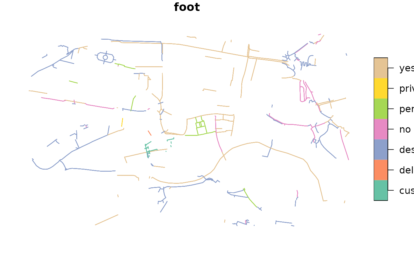
leeds_central %>% filter(foot == "yes") %>% select(foot) %>% plot() # returning only "yes" values in `foot`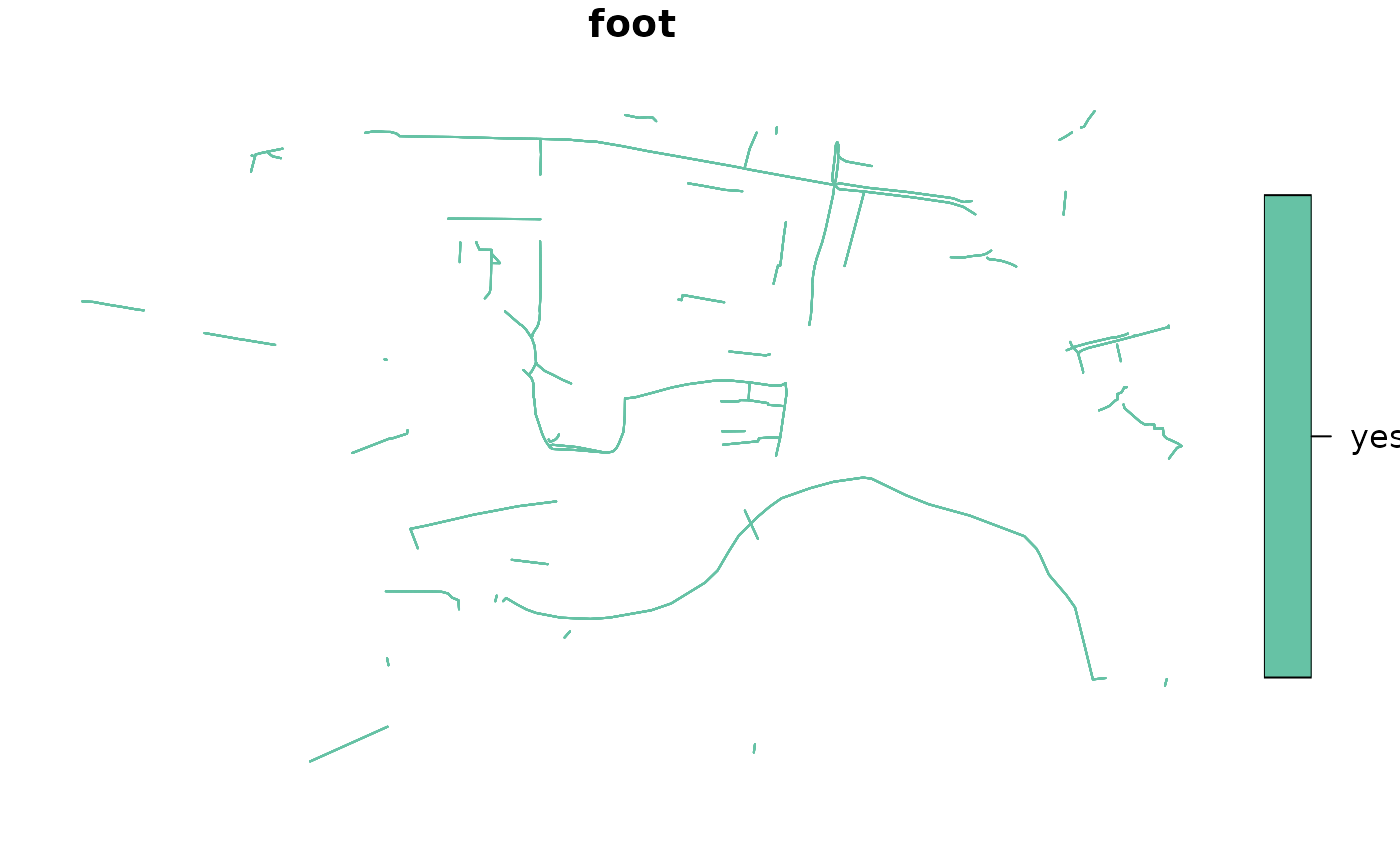
Interactive maps with tmap package
tmap is a
flexible package that allows to build both static and interactive maps
in R. In this section I will show you how to use its one-liner
qtm() (quick thematic maps) function to create interactive
maps (note: it might be code-efficient, but not always time-efficient!
It might take time to build maps, especially the large ones).
# first, we need to set out tmap mode to interactive
tmap::tmap_mode("view") # all the maps after this will be interactive
leeds_interactive = leeds_central %>%
  filter(!is.na(foot)) %>%
  select(foot) %>%
  tmap::qtm() # add `qtm()` at the end of to visualise your data
leeds_interactive
# if you want to your map to represent different types of foot values, then an additional `lines.col` argument is needed
leeds_interactive_color = leeds_central %>%
  filter(!is.na(foot)) %>%
  select(foot) %>%
  tmap::qtm(lines.col = "foot")
leeds_interactive_color
You might be wondering if you can plot static maps using
qtm() and the answer is yes.
tmap_mode("plot") # all the maps after this will be static
leeds_central %>%
  filter(!is.na(foot)) %>%
  select(foot) %>%
  tmap::qtm(lines.col = "foot")
Saving
# to save a map as html in your working directory
tmap::tmap_save(leeds_interactive, # a tmap object
          "leeds_interactive.html") # a name of a new .html file
Further reading
- Geocomputation with R for introduction to spatial analysis in R
- “Introducing osmextract” vignette for downloading OSM data
-
“tmap:
get started!” vignette or book-in-progress on
mapping with
tmappackage
Bibliography
Code for central Leeds can be found here: https://github.com/udsleeds/openinfra/blob/main/test-code/central%20leeds.R↩︎